Base R Statistics
Last updated: 2020-05-22
Checks: 6 1
Knit directory: R-codes/
This reproducible R Markdown analysis was created with workflowr (version 1.6.2). The Checks tab describes the reproducibility checks that were applied when the results were created. The Past versions tab lists the development history.
The R Markdown file has unstaged changes. To know which version of the R Markdown file created these results, you’ll want to first commit it to the Git repo. If you’re still working on the analysis, you can ignore this warning. When you’re finished, you can run wflow_publish to commit the R Markdown file and build the HTML.
Great job! The global environment was empty. Objects defined in the global environment can affect the analysis in your R Markdown file in unknown ways. For reproduciblity it’s best to always run the code in an empty environment.
The command set.seed(20200515) was run prior to running the code in the R Markdown file. Setting a seed ensures that any results that rely on randomness, e.g. subsampling or permutations, are reproducible.
Great job! Recording the operating system, R version, and package versions is critical for reproducibility.
Nice! There were no cached chunks for this analysis, so you can be confident that you successfully produced the results during this run.
Great job! Using relative paths to the files within your workflowr project makes it easier to run your code on other machines.
Great! You are using Git for version control. Tracking code development and connecting the code version to the results is critical for reproducibility.
The results in this page were generated with repository version a64008d. See the Past versions tab to see a history of the changes made to the R Markdown and HTML files.
Note that you need to be careful to ensure that all relevant files for the analysis have been committed to Git prior to generating the results (you can use wflow_publish or wflow_git_commit). workflowr only checks the R Markdown file, but you know if there are other scripts or data files that it depends on. Below is the status of the Git repository when the results were generated:
Ignored files:
    Ignored:    .RData
    Ignored:    .Rhistory
    Ignored:    .Rproj.user/

Unstaged changes:
    Modified:   analysis/base_r.Rmd
Note that any generated files, e.g. HTML, png, CSS, etc., are not included in this status report because it is ok for generated content to have uncommitted changes.
These are the previous versions of the repository in which changes were made to the R Markdown (analysis/base_r.Rmd) and HTML (docs/base_r.html) files. If you’ve configured a remote Git repository (see ?wflow_git_remote), click on the hyperlinks in the table below to view the files as they were in that past version.
| File | Version | Author | Date | Message |
|---|---|---|---|---|
| Rmd | a64008d | KaranSShakya | 2020-05-22 | base r: monte carlo |
| html | a64008d | KaranSShakya | 2020-05-22 | base r: monte carlo |
| html | 25d343a | KaranSShakya | 2020-05-20 | ggplot faceting |
| Rmd | 2da8824 | KaranSShakya | 2020-05-20 | adding to base r stat. |
| html | 2da8824 | KaranSShakya | 2020-05-20 | adding to base r stat. |
| html | e1a5784 | KaranSShakya | 2020-05-19 | link on all pages |
| Rmd | 9097ee4 | KaranSShakya | 2020-05-19 | aes erros SOLVED + links |
| html | 9097ee4 | KaranSShakya | 2020-05-19 | aes erros SOLVED + links |
| Rmd | 1a7c01c | KaranSShakya | 2020-05-19 | bug commit |
| Rmd | a286ee6 | KaranSShakya | 2020-05-18 | normal dist |
| html | a286ee6 | KaranSShakya | 2020-05-18 | normal dist |
| Rmd | c42059f | KaranSShakya | 2020-05-16 | base r analysis - first drafts |
| html | c42059f | KaranSShakya | 2020-05-16 | base r analysis - first drafts |
Generating sequences
Normal sequence
x <- seq(1:10)
x
[1] 1 2 3 4 5 6 7 8 9 10Odd numbers only
x.odd <- seq(1,10,2)
x.odd
[1] 1 3 5 7 9Even distribution between ranges. Example: 3 equal division between 1 and 10.
y.divide <- seq(1,10, length.out = 3)
y.divide
[1] 1.0 5.5 10.0Monte Carlo Simulations
Discrete
Monte Carlo simulations model the probability of different outcomes by repeating a random process a large enough number of times that the results are similar to what would be observed if the process were repeated forever. First, create an box with data. This can be done through rep (2 red, 3 blue balls:
beads <- rep(c("red", "blue"), times = c(2,3))
beads
[1] "red" "red" "blue" "blue" "blue"Lets pick a bead from this box 10,000 times. To do this, we set up B and run it.
B <- 100000
events <- replicate(B, sample(beads, 1))    # draw 1 bead, B times
tab <- table(events)    # make a table of outcome counts
prop.table(tab)    # view table of outcome proportio
events
blue red
0.60104 0.39896 Continuous
Generating simulated height data using normal distribution.
x <- heights %>% filter(sex=="Male") %>% pull(height)
n <- length(x)
avg <- mean(x)
s <- sd(x)
simulated_heights <- rnorm(n, avg, s)
The sumulated_heights is built from the length, mena, and sd. The plot of this is as follows. Important to note that this is built from the assumption of normal distribution:
data.frame(simulated_heights = simulated_heights) %>%
ggplot(aes(simulated_heights)) +
geom_histogram(color="black", binwidth = 2)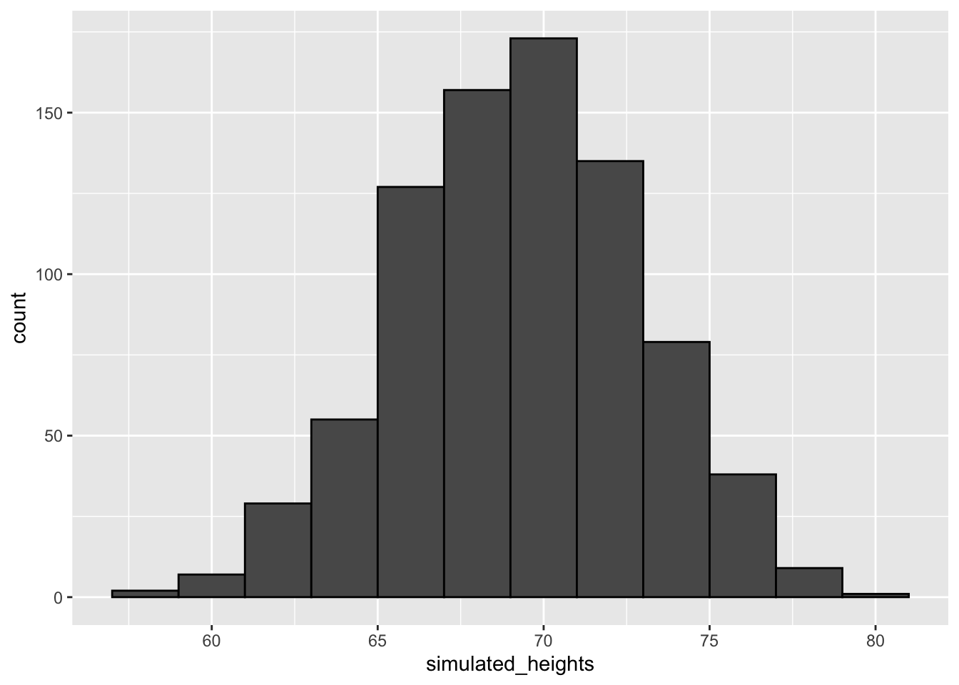 Example, running a monte carlo simulation to find out the probablity of people over 7 feet (answer: 0.0214). Running the simulation 10,000 times (B):
set.seed(3233)
B <- 10000
tallest <- replicate(B, {
    simulated_data <- rnorm(800, avg, s)    # generate 800 normally distributed random heights
    max(simulated_data)    # determine the tallest height
})
mean(tallest >= 7*12) #7*12 = 84 inches, which is 7 feet.
[1] 0.0214Important to note the set.seed() function allows us to control the random. Without this function, the answer would be different because you cannot control the random variability. But with set.seed() you will have the same answer every time.
Mean / Sd
For mean, median, sd, min, max:
heights %>%
    filter(sex == "Male") %>%
    summarize(average=mean(height), sd=sd(height), median = median(height),
              minimum = min(height), maximum = max(height))
Observing Columns
murders is the dataset. To observe the column types,
str(murders)'data.frame': 51 obs. of 5 variables:
$ state : chr "Alabama" "Alaska" "Arizona" "Arkansas" ...
$ abb : chr "AL" "AK" "AZ" "AR" ...
$ region : Factor w/ 4 levels "Northeast","South",..: 2 4 4 2 4 4 1 2 2 2 ...
$ population: num 4779736 710231 6392017 2915918 37253956 ...
$ total : num 135 19 232 93 1257 ...To observe all column numbers. Easy to see which column is which number.
names(murders)[1] "state" "abb" "region" "population" "total" To observe the first 5 data data of a column.
murders$state[1:5][1] "Alabama" "Alaska" "Arizona" "Arkansas" "California"Data Frames (Vectors)
Associating vectors only
city <- c("Tokyo", "Lile", "Dover")
area <- c(10, 8, 13)
names(area) <- city
area
Tokyo Lile Dover
10 8 13 Creating Data Frames. Extra column created because of previous code.
data <- data.frame(name=city, value=area)
data
name value
Tokyo Tokyo 10
Lile Lile 8
Dover Dover 13Normal Distribution
q-q graph
To see if male dataset follow a normal distribution. First define p as quantile ranges from 0.05 to 0.95.
p <- seq(0.05, 0.95, 0.05)The observed_q is the real quantile of your dataset. The theory_q is the expected quantiles of a normal distribution.
observed_q <- quantile(male$height, p)
theory_q <- qnorm(p, mean=mean(male$height), sd=sd(male$height))
The see closely they match, simply plot them. This shows that points almost match, so male dataset is a good approximation for normal distribution. 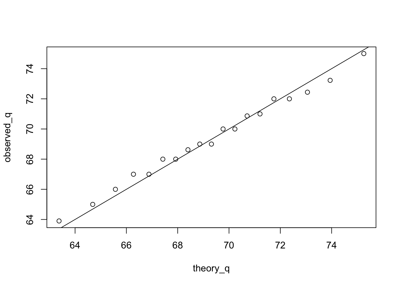 ***
***
sessionInfo()R version 4.0.0 (2020-04-24)
Platform: x86_64-apple-darwin17.0 (64-bit)
Running under: macOS Catalina 10.15.4
Matrix products: default
BLAS: /Library/Frameworks/R.framework/Versions/4.0/Resources/lib/libRblas.dylib
LAPACK: /Library/Frameworks/R.framework/Versions/4.0/Resources/lib/libRlapack.dylib
locale:
[1] en_US.UTF-8/en_US.UTF-8/en_US.UTF-8/C/en_US.UTF-8/en_US.UTF-8
attached base packages:
[1] stats graphics grDevices utils datasets methods base
other attached packages:
[1] dslabs_0.7.3 forcats_0.5.0 stringr_1.4.0 dplyr_0.8.5
[5] purrr_0.3.4 readr_1.3.1 tidyr_1.0.3 tibble_3.0.1
[9] ggplot2_3.3.0 tidyverse_1.3.0 workflowr_1.6.2
loaded via a namespace (and not attached):
[1] tidyselect_1.1.0 xfun_0.13 haven_2.2.0 lattice_0.20-41
[5] colorspace_1.4-1 vctrs_0.3.0 generics_0.0.2 htmltools_0.4.0
[9] yaml_2.2.1 rlang_0.4.6 later_1.0.0 pillar_1.4.4
[13] withr_2.2.0 glue_1.4.1 DBI_1.1.0 dbplyr_1.4.3
[17] modelr_0.1.7 readxl_1.3.1 lifecycle_0.2.0 munsell_0.5.0
[21] gtable_0.3.0 cellranger_1.1.0 rvest_0.3.5 evaluate_0.14
[25] labeling_0.3 knitr_1.28 httpuv_1.5.2 fansi_0.4.1
[29] broom_0.5.6 Rcpp_1.0.4.6 promises_1.1.0 backports_1.1.6
[33] scales_1.1.1 jsonlite_1.6.1 farver_2.0.3 fs_1.4.1
[37] hms_0.5.3 digest_0.6.25 stringi_1.4.6 grid_4.0.0
[41] rprojroot_1.3-2 cli_2.0.2 tools_4.0.0 magrittr_1.5
[45] crayon_1.3.4 whisker_0.4 pkgconfig_2.0.3 ellipsis_0.3.0
[49] xml2_1.3.2 reprex_0.3.0 lubridate_1.7.8 rstudioapi_0.11
[53] assertthat_0.2.1 rmarkdown_2.1 httr_1.4.1 R6_2.4.1
[57] nlme_3.1-147 git2r_0.27.1 compiler_4.0.0