Data Visualization
Last updated: 2020-05-21
Checks: 6 1
Knit directory: R-codes/
This reproducible R Markdown analysis was created with workflowr (version 1.6.2). The Checks tab describes the reproducibility checks that were applied when the results were created. The Past versions tab lists the development history.
The R Markdown file has unstaged changes. To know which version of the R Markdown file created these results, you’ll want to first commit it to the Git repo. If you’re still working on the analysis, you can ignore this warning. When you’re finished, you can run wflow_publish to commit the R Markdown file and build the HTML.
Great job! The global environment was empty. Objects defined in the global environment can affect the analysis in your R Markdown file in unknown ways. For reproduciblity it’s best to always run the code in an empty environment.
The command set.seed(20200515) was run prior to running the code in the R Markdown file. Setting a seed ensures that any results that rely on randomness, e.g. subsampling or permutations, are reproducible.
Great job! Recording the operating system, R version, and package versions is critical for reproducibility.
Nice! There were no cached chunks for this analysis, so you can be confident that you successfully produced the results during this run.
Great job! Using relative paths to the files within your workflowr project makes it easier to run your code on other machines.
Great! You are using Git for version control. Tracking code development and connecting the code version to the results is critical for reproducibility.
The results in this page were generated with repository version d65de39. See the Past versions tab to see a history of the changes made to the R Markdown and HTML files.
Note that you need to be careful to ensure that all relevant files for the analysis have been committed to Git prior to generating the results (you can use wflow_publish or wflow_git_commit). workflowr only checks the R Markdown file, but you know if there are other scripts or data files that it depends on. Below is the status of the Git repository when the results were generated:
Ignored files:
    Ignored:    .RData
    Ignored:    .Rhistory
    Ignored:    .Rproj.user/

Unstaged changes:
    Modified:   analysis/data_visualization.Rmd
Note that any generated files, e.g. HTML, png, CSS, etc., are not included in this status report because it is ok for generated content to have uncommitted changes.
These are the previous versions of the repository in which changes were made to the R Markdown (analysis/data_visualization.Rmd) and HTML (docs/data_visualization.html) files. If you’ve configured a remote Git repository (see ?wflow_git_remote), click on the hyperlinks in the table below to view the files as they were in that past version.
| File | Version | Author | Date | Message |
|---|---|---|---|---|
| Rmd | b1dee72 | KaranSShakya | 2020-05-21 | data visualiaztion commits |
| html | b1dee72 | KaranSShakya | 2020-05-21 | data visualiaztion commits |
| Rmd | 25d343a | KaranSShakya | 2020-05-20 | ggplot faceting |
| html | 25d343a | KaranSShakya | 2020-05-20 | ggplot faceting |
| Rmd | 2b4e76b | KaranSShakya | 2020-05-19 | final data visualization (for now) |
| html | 2b4e76b | KaranSShakya | 2020-05-19 | final data visualization (for now) |
| Rmd | 9097ee4 | KaranSShakya | 2020-05-19 | aes erros SOLVED + links |
| html | 9097ee4 | KaranSShakya | 2020-05-19 | aes erros SOLVED + links |
| Rmd | 99962e5 | KaranSShakya | 2020-05-19 | bug aes error - 1 |
| Rmd | 1a7c01c | KaranSShakya | 2020-05-19 | bug commit |
| Rmd | 27ba057 | KaranSShakya | 2020-05-17 | update ggplots + data for it |
| html | 27ba057 | KaranSShakya | 2020-05-17 | update ggplots + data for it |
Histogram
Histogram. Change binwidth to alter the shape of the slopes. 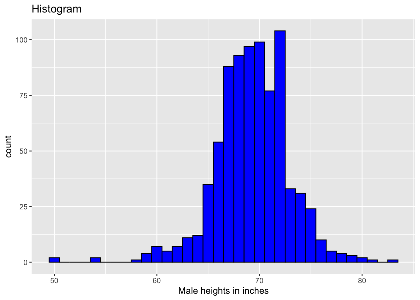
| Version | Author | Date |
|---|---|---|
| 2b4e76b | KaranSShakya | 2020-05-19 |
To create a smooth histogram (more similar to normal distribution graphs)
ggplot(hist, aes(x=height))+
  geom_density(fill = "green2")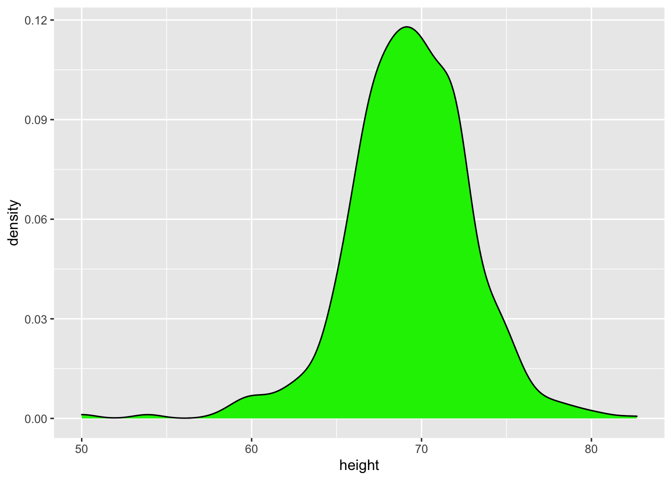
Histogram (different bin levels)
gg.arrange used to see how different binwidth affects different histograms. Needs package gridExtra.
p <- heights %>% filter(sex == "Male") %>% ggplot(aes(x = height))
p1 <- p + geom_histogram(binwidth = 1, fill = "blue", col = "black")
p2 <- p + geom_histogram(binwidth = 2, fill = "blue", col = "black")
p3 <- p + geom_histogram(binwidth = 3, fill = "blue", col = "black")

grid.arrange(p1, p2, p3, ncol = 3)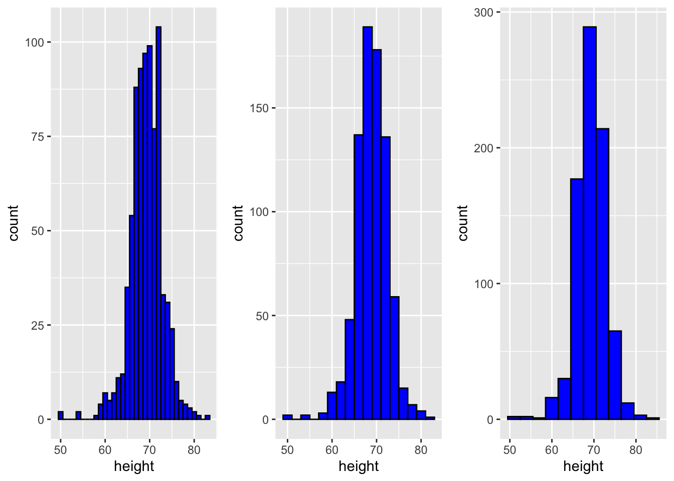
| Version | Author | Date |
|---|---|---|
| 2b4e76b | KaranSShakya | 2020-05-19 |
Q-Q Plot
Basic qq plot:
p1 <- heights %>% filter(sex == "Male")
ggplot(p1, aes(sample = height))+
  geom_qq()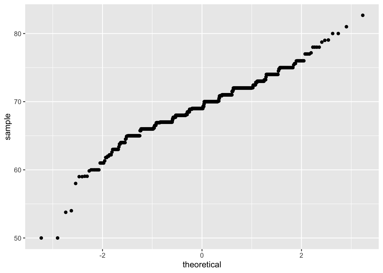
Boxed Plot
Stacked Box Plot with Reorder
This stacked box plot is log scaled.
gapminder %>%
    filter(year == "1970" & !is.na(gdp)) %>%
    mutate(region = reorder(region, dollars_per_day, FUN = median)) %>%    # reorder
    ggplot(aes(region, dollars_per_day, fill = continent)) +    # color by continent
    geom_boxplot() +
    theme(axis.text.x = element_text(angle = 90, hjust = 1)) +
    xlab("")+
  scale_y_continuous(trans = "log2")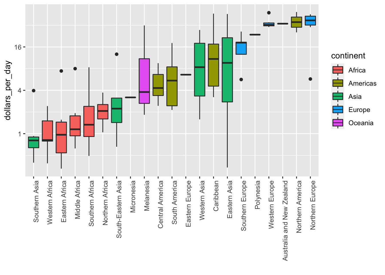
| Version | Author | Date |
|---|---|---|
| b1dee72 | KaranSShakya | 2020-05-21 |
Line Plot
ggplot(LAC, aes(x=Year))+
  geom_line(aes(y=Yield_r), color="Green3", size=1)+
  geom_line(aes(y=Area_r), color="Green3", linetype="dashed", size=1)+
  labs(title="Latin America & Caribbean", x="Year", y="Relative Change")+
  theme_bw(base_size = 12)+
  coord_cartesian(ylim=c(80, 140))+
  scale_y_continuous(breaks = seq(80, 140, 10))+
  scale_x_continuous(breaks = seq(2002, 2016, 2))+
  geom_segment(aes(x=2002, y=100, xend=2016, yend=100), size=0.5)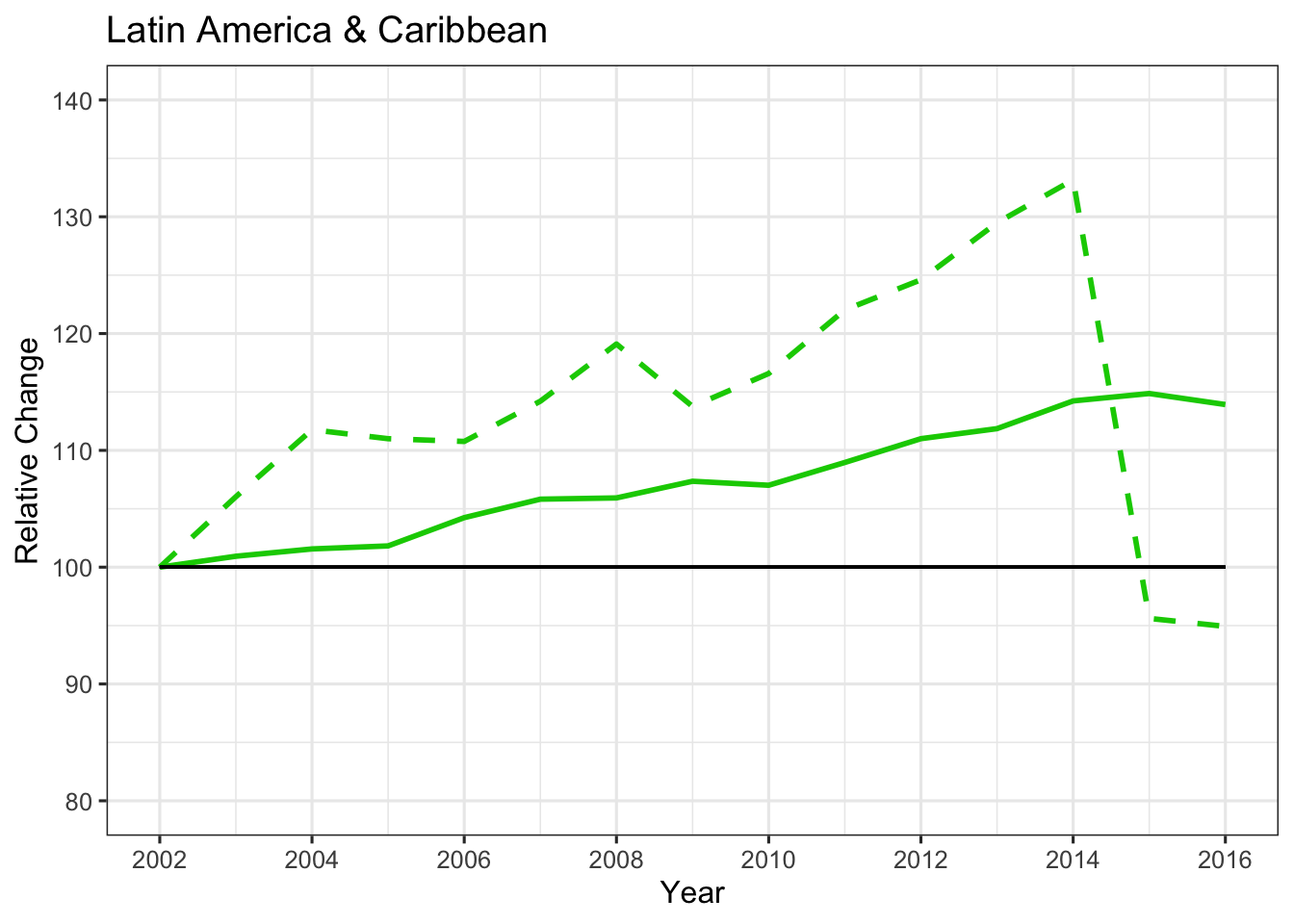
countries <- c("South Korea", "Germany")
new_labels <- data.frame(country = countries, x = c(1975, 1965), y = c(60, 72))

gapminder %>% filter(country %in% countries) %>%
    ggplot(aes(year, life_expectancy, col = country)) +
    geom_line() +
    geom_text(data = new_labels, aes(x, y, label = country), size = 5) +
    theme(legend.position = "none")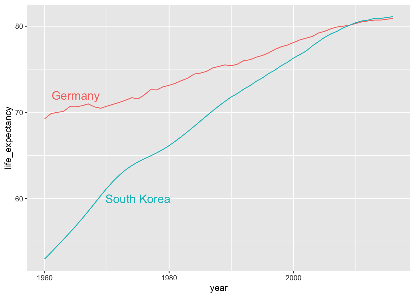
| Version | Author | Date |
|---|---|---|
| b1dee72 | KaranSShakya | 2020-05-21 |
Scatterplot
Harvard Course Example
First a code to calculate summary statistics to put on graph.
summary_r <- murders %>%
    summarize(rate = sum(total) / sum(population) * 10^6) %>%
    .$rate
The code for plot:
ggplot(murders, aes(x=population/10^6, y=total, label = abb)) +
    geom_abline(intercept = log10(summary_r), lty = 2, color = "darkgrey") +
    geom_point(aes(col = region), size = 3) +
    geom_text_repel() +
    scale_x_log10() +
    scale_y_log10() +
    labs(title = "US Gun Murders in 2010", x="Population in millions (log scale)",
         y="Total number of murders (log scale)")+
    scale_color_discrete(name = "Region") +
    theme_economist()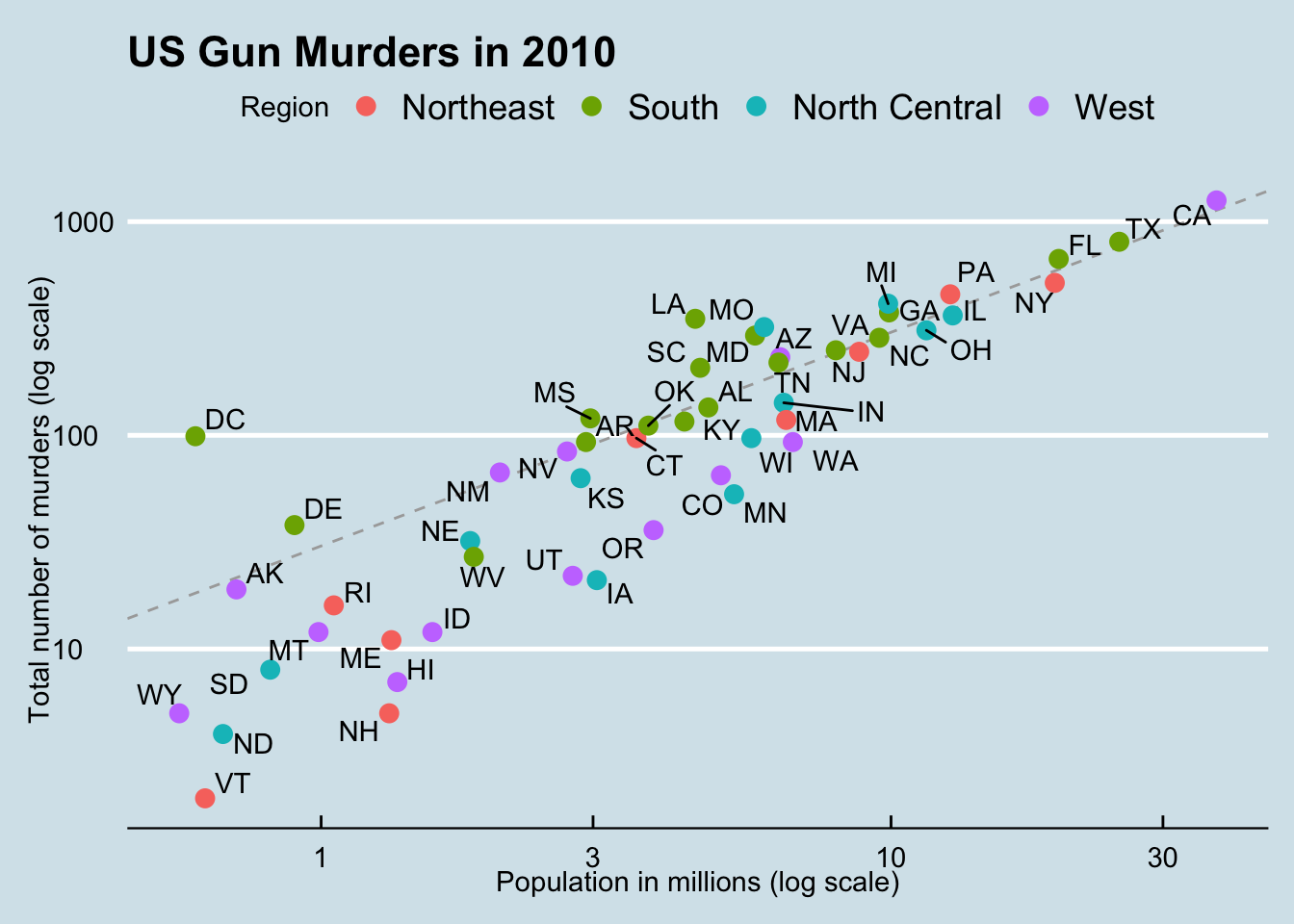
Country - Name
ggplot(data2, aes(x=log(GDP_capita), y=log(Fertilizer_use), color=Region))+
  geom_point()+
  geom_text(aes(label=Country), hjust=1, vjust=0)+
  labs(title="Fertilizer Use (2016)", x="Log(GDP per Capita)", y="Log(Fertilizer Use)")+
  theme_classic(base_size = 12)+
  coord_cartesian(xlim=c(5.5, 11.2))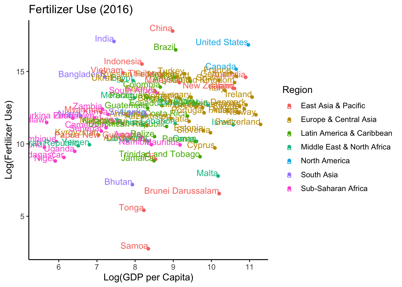
Faceting
Faceting is important in comparing or in showing trends. Benefit is that the scale is same which makes comparison easier. The first graph is for 2 variables (continent ~ year).
filter(gapminder, year %in% c(1962, 2012)) %>%
    ggplot(aes(fertility, life_expectancy, col = continent)) +
    geom_point() +
    facet_grid(continent ~ year)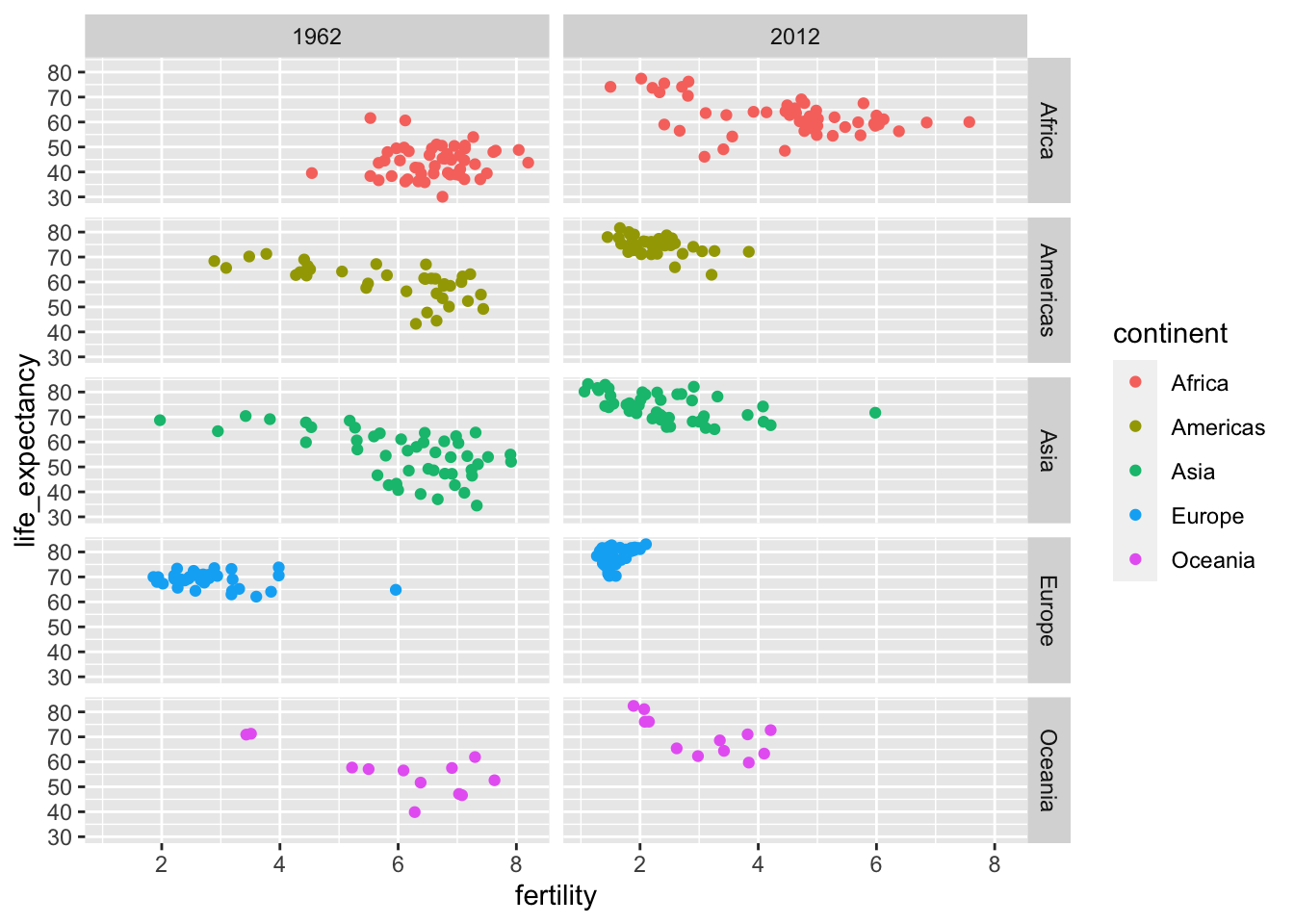
| Version | Author | Date |
|---|---|---|
| b1dee72 | KaranSShakya | 2020-05-21 |
This one is only for one variable (. ~ year).
filter(gapminder, year %in% c(1962, 2012)) %>%
    ggplot(aes(fertility, life_expectancy, col = continent)) +
    geom_point() +
    facet_grid(. ~ year)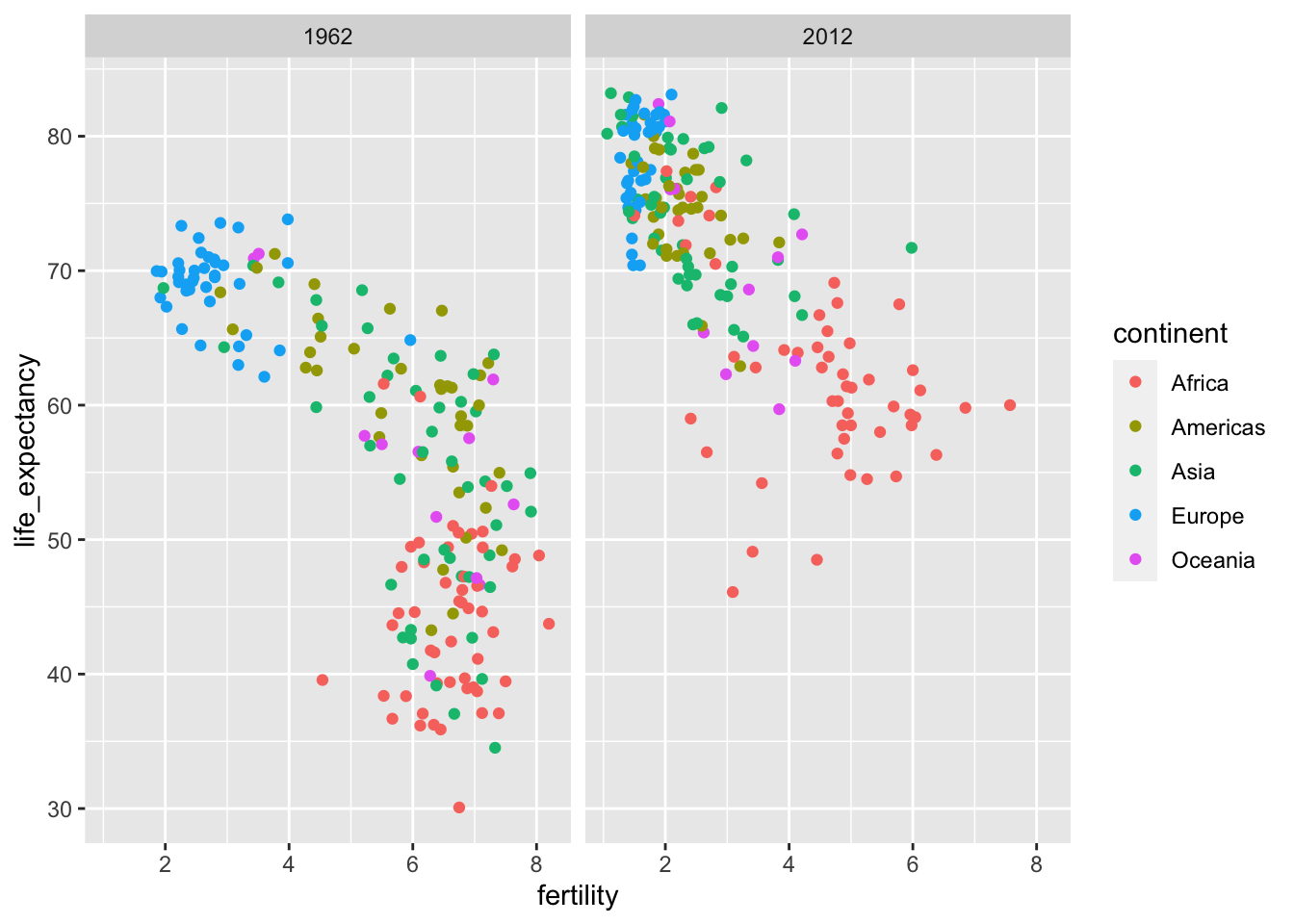
| Version | Author | Date |
|---|---|---|
| b1dee72 | KaranSShakya | 2020-05-21 |
For specifc comparion example:
years <- c(1962, 1980, 1990, 2000, 2012)
continents <- c("Europe", "Asia")
gapminder %>%
    filter(year %in% years & continent %in% continents) %>%
    ggplot(aes(fertility, life_expectancy, col = continent)) +
    geom_point() +
    facet_wrap(~year)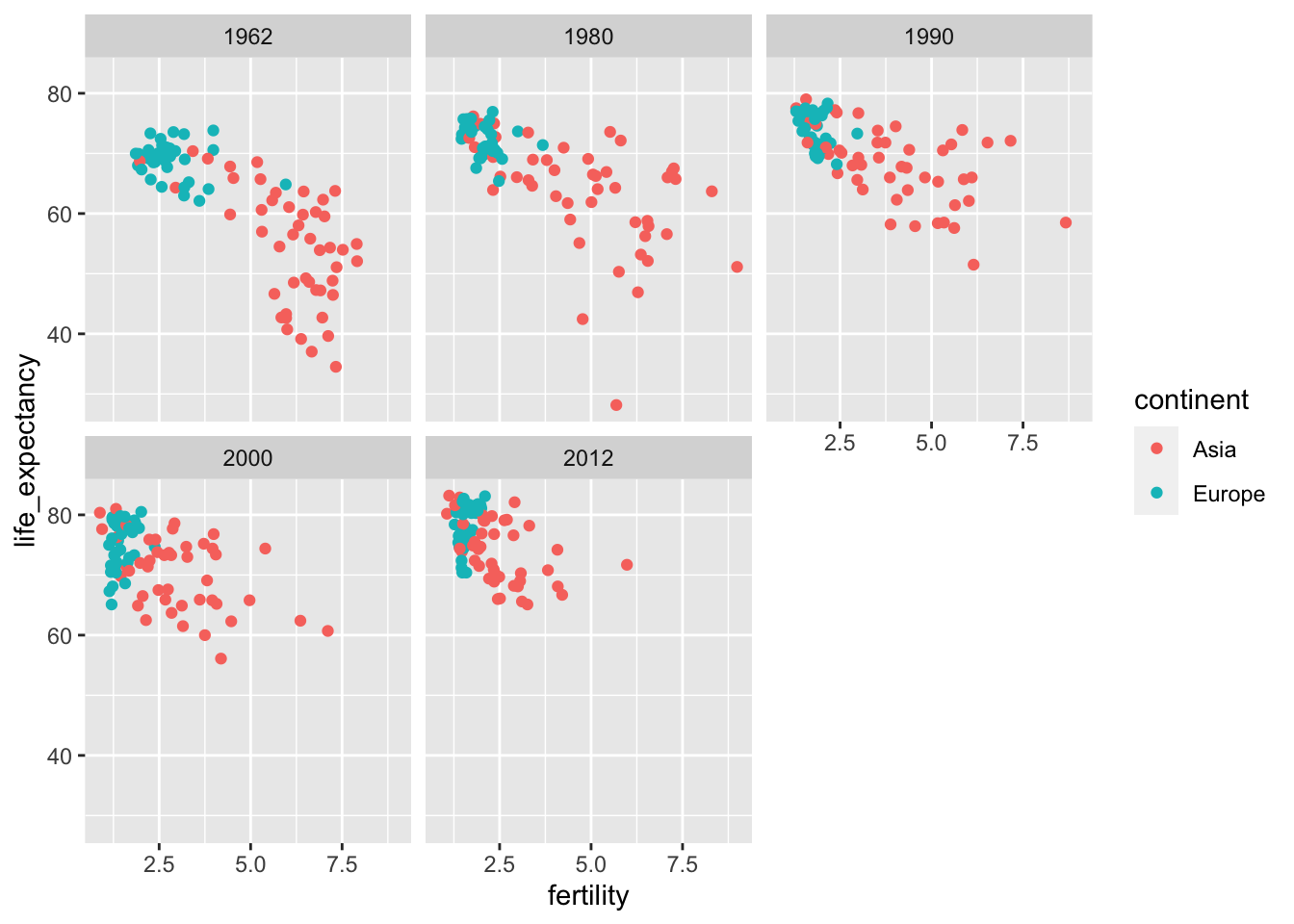
| Version | Author | Date |
|---|---|---|
| b1dee72 | KaranSShakya | 2020-05-21 |
sessionInfo()R version 4.0.0 (2020-04-24)
Platform: x86_64-apple-darwin17.0 (64-bit)
Running under: macOS Catalina 10.15.4
Matrix products: default
BLAS: /Library/Frameworks/R.framework/Versions/4.0/Resources/lib/libRblas.dylib
LAPACK: /Library/Frameworks/R.framework/Versions/4.0/Resources/lib/libRlapack.dylib
locale:
[1] en_US.UTF-8/en_US.UTF-8/en_US.UTF-8/C/en_US.UTF-8/en_US.UTF-8
attached base packages:
[1] stats graphics grDevices utils datasets methods base
other attached packages:
[1] dslabs_0.7.3 ggthemes_4.2.0 ggrepel_0.8.2 gridExtra_2.3
[5] forcats_0.5.0 stringr_1.4.0 dplyr_0.8.5 purrr_0.3.4
[9] readr_1.3.1 tidyr_1.0.3 tibble_3.0.1 ggplot2_3.3.0
[13] tidyverse_1.3.0 readxl_1.3.1 workflowr_1.6.2
loaded via a namespace (and not attached):
[1] Rcpp_1.0.4.6 lubridate_1.7.8 lattice_0.20-41 assertthat_0.2.1
[5] rprojroot_1.3-2 digest_0.6.25 R6_2.4.1 cellranger_1.1.0
[9] backports_1.1.6 reprex_0.3.0 evaluate_0.14 httr_1.4.1
[13] pillar_1.4.4 rlang_0.4.6 rstudioapi_0.11 whisker_0.4
[17] rmarkdown_2.1 labeling_0.3 munsell_0.5.0 broom_0.5.6
[21] compiler_4.0.0 httpuv_1.5.2 modelr_0.1.7 xfun_0.13
[25] pkgconfig_2.0.3 htmltools_0.4.0 tidyselect_1.1.0 fansi_0.4.1
[29] crayon_1.3.4 dbplyr_1.4.3 withr_2.2.0 later_1.0.0
[33] grid_4.0.0 nlme_3.1-147 jsonlite_1.6.1 gtable_0.3.0
[37] lifecycle_0.2.0 DBI_1.1.0 git2r_0.27.1 magrittr_1.5
[41] scales_1.1.1 cli_2.0.2 stringi_1.4.6 farver_2.0.3
[45] fs_1.4.1 promises_1.1.0 xml2_1.3.2 ellipsis_0.3.0
[49] generics_0.0.2 vctrs_0.3.0 tools_4.0.0 glue_1.4.1
[53] hms_0.5.3 yaml_2.2.1 colorspace_1.4-1 rvest_0.3.5
[57] knitr_1.28 haven_2.2.0